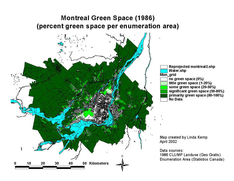
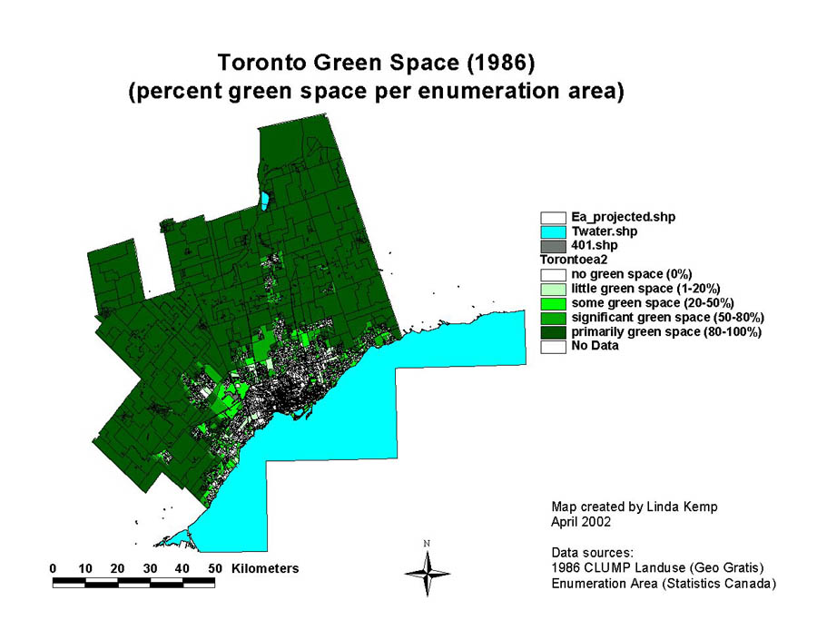
A raster based analysis was used to analyze the maps and consequently, the land cover maps were converted into grids. Figures 1 and 2 show the land cover grids, with the EA polygons layered on top. It should be noted that due to the complex nature (the program would crash) of the river polygons on the Montreal map, and the highway polygons on the Toronto maps, these elements were not included on the final grids. This was later accounted for.
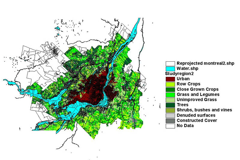
Montreal land cover with enumeration area polygons

Toronto land cover with enumeration area polygons
The next step in the analysis was to convert the enumeration area maps into grids. The first grid (EA_Grid_A) was made was based on the unique EA number of each polygon. This way the pixels of the grid each represented the value of the EA that the area belonged to and the original format of the EA table was not changed. Following, the Microsoft Access query table was joined to the EA_Grid_A theme table, using EA as a common field, in order to show the number of houses built in each EA.
To properly analyze the green space conversion into new housing, the EA_Grid_A table for each city needed to include the following information:
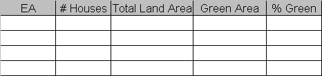
At this point in time ‘EA’ and ‘# Houses’ was known. Obtaining the ‘% Green’ would be a bit harder, especially since I had to assign 100% values for many of the EAs.
The first step in obtaining ‘% Green’ was to determine the Total Land Area. For Toronto this could be done simply by calculating the area for each EA. Unfortunately though, for Montreal it was a bit more difficult since EA areas included the river. Instead the Montreal areas were determined using the Tabulate Areas function with the EA_Grid_A map and the Land cover map. To simplify the result, a Boolean column was added to the Land cover map, with every value being True. This way the Tabulate Areas function returned one total area and not the area of each of each individual cover type. Another problem encountered at this time was that the land cover map did not line up perfectly with the EA map (as shown below). This meant that the area calculated was incorrect for EA areas that did not have full land cover information, or that had no land cover information.
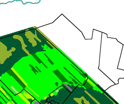
This included over 100 polygons and so to take this into account a new grid had to be created. The new grid (EA_Grid_ B) was created which represented only the area that overlapped the land cover map. This was made by deleting all the polygons of the EA vector map (a copy of the original EA vector map) that did not lie atop the land cover map. The resulting map was converted then into a grid, again with EA number as the pixel value. The Tabulate Areas function was used again, but this time it only produced area values for areas with full land cover information.
The next step was to calculate the ‘Green Area’. For this, a query was done on the land cover map, which showed only areas that were classified as green areas. This included: row crops; close grown crops; improved grass and legumes; unimproved grassland, reeds, sedges, mosses and other non-woody plants; trees; and shrubs, bushes and vines. The resulting selection was then converted into a grid, and again a Boolean column was added to the table with all values being “True”. The Tabulate Areas function was used to determine ‘Green Area’ for each EA and subsequently the ‘% Green’ was calculated as ‘Green Area’ / ‘Total Land Area’. For Montreal, the EA_Grid_B was then joined back to EA_Grid_A. This of course only provided the ‘% Green’ area that was within the land cover region. For the analysis, everything outside of the land cover region was to be assumed 100% green and thus the table had to be modified. Due to the number of records (>5000) in the table, manual data entry was not an option. Some manual manipulation of the records was however done to the Toronto table. This was done in order to correct faulty values that arose in the calculation of ‘Green Area’ for Toronto. As with Montreal, the slight overlap error between the Land cover map and EA map creates faulty area values. This time manual manipulation was viable since very few of Toronto’s EAs encountered this problem.
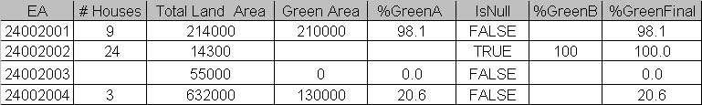
To assign a 100% green area to EA areas outside the Land cover region, a table similar to the example below, was created and ‘%Green’ was renamed ‘%GreenA’. As you can see for ‘EA’ 24002002, there was a null value for ‘Green Area’, and thus also for ‘%GreenA’. A Boolean column, IsNull, was then made which showed fields where ‘%GreenA’ had a null value. Next, as query was done to select records that were True for this column and these records were subsequently turned into a new map showing all of the areas outside the land cover region. Using the theme table, each EA was then assigned a “%GreenB” value of 100%. Following, the table was rejoined back to the EA_Grid_A theme table using EA as a common field. A column %GreenFinal, which now included a record for every EA, could now be calculated as the sum of %GreenA and %GreenB. For this calculation, the table was exported into Excel in order to assign empty cells with a value of zero. The result was then imported back into ArcView and joined to the EA_Grid _A table
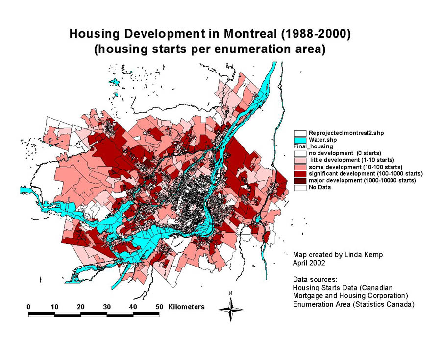
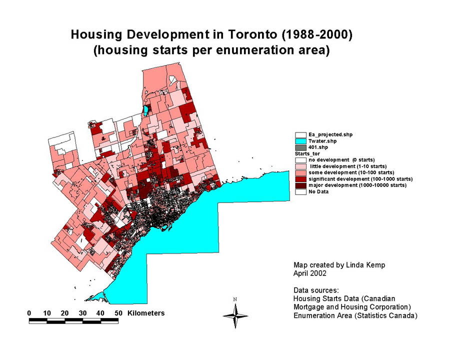
Using the values in the above theme table, the EA_Grid_A could now be modified to show ‘#Houses’ or ‘%GreenFinal’ simply by changing the legend. The figures below show the final maps made from ‘# Houses’ and ‘%GreenFinal’ for each city.
The next step of the analysis was to reclassify the maps so that a comparison could be made. Using the Reclassify function in ArcView, each of the four above maps was reclassified into the categories described in the legend. At this time I had hoped to export my data into IDRISI where I could create a Cross Tabulate Areas map for the reclassified EAs. However, due to the complex nature of the grids, this was not an option. Instead, using the Tabulate Areas function in ArcView a table was created in order to quantify land conversion of green space into new housing. The table was then imported into Excel where the values were modified into units of percent of total area, instead of square meters. This allowed for a comparison to be made between the two cities of different size.
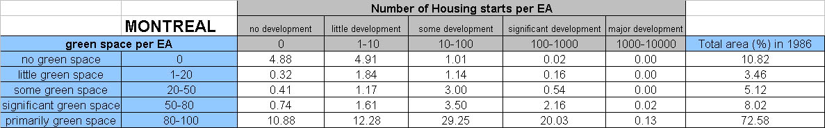

In general, the results of the table do not clearly show either city to have conserved more green space than the other. While Toronto had more major developments (>1000 houses per EA) on primarily green space, Montreal had more significant developments (100-1000 houses per EA). Thus, using these tables, two final graphs and a comparison table were created to better visualize and understand the results.

From the above graph it is obvious that neither Montreal nor Toronto have been particularly concerned about conserving green space. Both cities have shown a significant amount of new housing development is taking place in regions that were previously 100% green, though Montreal’s primarily green space consumption was slightly lower.

The above graph displays the development patterns for new housing which was again quite similar for both cities. In both cases the number of new houses built in an enumeration area was typically of the class “some development” which described 100-1000 houses over the study period. It was fairly uncommon for an enumeration area to have major development (greater than 1000 houses built over the study period) though this occurred more often in Toronto than in Montreal.

Finally, the above table directly compares the landuse conversion for each city. And, since there is no clear evidence from this study as to which city was more environmentally friendly, lets try a less scientific approach - just to get some idea. From the table it can be seen that Montreal left a greater percentage of primarily green space untouched - so lets consider that one point for Montreal. However Toronto left more significantly green areas untouched (1:1). Next, Montreal has less primarily green areas with major development so its 2:1 for Montreal. But, Toronto gets another point for having less significant development of primarily green areas (2:2). Montreal scores another point for having less primarily green areas with some development (3:2), and another for having less significantly green areas with significant development (4:2). And, Montreal gets yet one more point for having less significantly green areas with significant development (5:2). However, Toronto proves to be a fierce competitor in the last two categories having less significantly green areas with some development (5:3) and finally by having a greater percentage of primarily and significantly green areas with little or no development, though the numbers in this category are extremely close. Which brings us to a final score 5:4 or Montreal - still not very convincing.
Overall the answer to "Which city converted the least amount of green space into new housing?" is still unclear. As mentioned above, while Toronto had more major developments (>1000 houses per EA) on primarily green space, Montreal had more significant developments (100-1000 houses per EA). Montreal seemed to have made smaller developments in areas with slightly less green space, but it’s likely that the developments made were still on green space. Toronto seemed to have a greater tendency to clear-cut green areas and create very densely populated new housing developments. It is hard to argue if one way is better than the other. If I had to pick I’d say that the results might suggest that Montreal was more responsible in its development, which is what I had expected. It should however be noted that, due to the classification type of analysis done here, it is possible that better defined classes would have provided much clearer results. As this study is of particular interest to Professor Haider, I expect that further analysis, and likely the reclassification of these results, will be preformed. For the present study, however, the jury is still out.
